How to Highlight Duplicates in Google Sheets (Conditional Formatting + COUNTIF)

A name that appears twice in a guest list or order sheet throws off every total. With ten rows you can spot it by eye, but with a few hundred it's easy to miss.

 

In Google Sheets you can combine conditional formatting with a single COUNTIF formula to color only the duplicate values. It updates automatically as you type new entries.

 

1. Select the range → Format → Conditional formatting

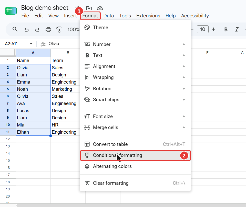
Select the range to check for duplicates. In this example it's the Name column, A2:A11. Then click ① Format → ② Conditional formatting.

 

Select A2:A11, then click Format → Conditional formatting

 

2. Enter a custom formula and pick a color

The Conditional format rules panel opens on the right with A2:A11 already in the range box.

 

Enter the COUNTIF formula as a custom formula and set a light red fill

 

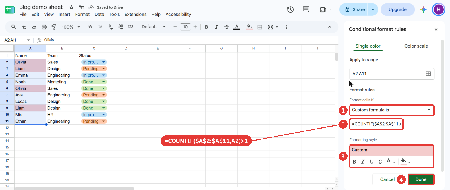
1. Open the Format cells if… list and choose Custom formula is at the very bottom.
2. Type the formula below into the value box.
3. Under Formatting style, change the fill color (paint bucket icon) to light red.
4. Click Done.

 

=COUNTIF($A$2:$A$11,A2)>1

 

3. Check the result

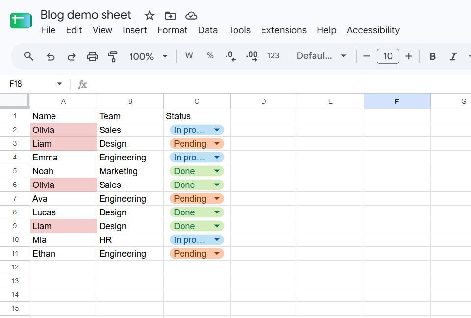
Only Olivia and Liam, the names that appear more than once, are highlighted.

 

Only the duplicate names (Olivia, Liam) are filled in light red

 

What the formula does

COUNTIF(range, value) counts how many times a value appears in a range.

 

• $A$2:$A$11: the whole range to compare against. The $ signs lock it, so every cell is counted against the same range.
• A2: the cell being checked. Without $ it shifts down to A3, A4, and so on for each row.
• >1: if the value appears two or more times (a duplicate), the result is TRUE and the cell gets colored.

 

Variations

• Check the whole column: set the range to A2:A and use =COUNTIF($A$2:$A,A2)>1 so new rows are checked too. To keep empty cells from being colored, use =AND(A2<>"",COUNTIF($A$2:$A,A2)>1).
• Highlight only the repeats: =COUNTIF($A$2:A2,A2)>1 leaves the first occurrence alone and colors only the later copies. Handy when you're deciding which rows to delete.
• Remove the rule: in the same panel, hover over the rule and click the trash icon.

 

📚 More Google Sheets tips

· How to Create a Dropdown List in Google Sheets NEW